Interactive workbench

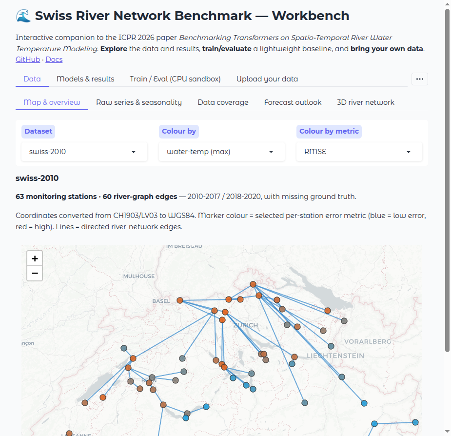
The workbench is a one-command, browser-based application for exploring the benchmark, training and evaluating quick baselines, running your own model, and analysing predictions — with an emphasis on being usable by hydrologists who do not want to write code. The same application powers both the hosted Hugging Face Space and the local app, from a single source file, so what you see online is exactly what you run locally.

• Local: uv run srn app gradio (or python -m swissrivernetwork.app.workbench)
• Hosted: open the Space — no install required.

Who is this for?

Two audiences are served side by side. Hydrologists and water managers get a map, seasonal cycles, a drought-portal-style outlook, and ecological threshold analysis without touching a line of code. ML researchers get the full result set (window-length, forecasting horizon, noise robustness, per-station error, radar, ranking) plus a bring-your-own-model inference and analysis workflow.

Launching it

One-click (no coding needed). Double-click scripts/launch-workbench.command (macOS) or scripts/launch-workbench.bat (Windows), or run scripts/launch-workbench.sh (Linux). It installs the uv package manager and all dependencies on the first run, then opens the app in your browser — nothing else to set up.

From the command line:

# Recommended: installs the app extra (gradio, folium, …) on first run.
uv run srn app gradio
# Equivalent:
uv run python -m swissrivernetwork.app.workbench

The app opens on http://127.0.0.1:7860. Useful environment variables:

Variable	Default	Meaning
SRN_HOST	0.0.0.0	Interface to bind. Set to 127.0.0.1 to keep it private to your machine.
SRN_PORT	7860	Port to serve on.
SRN_WORKBENCH_DATA	(bundled)	Path to an alternative data bundle. Overrides the packaged demo data.

Compute: CPU and GPU are detected automatically

The Inference tab shows the environment it detected — CPU cores, RAM, and, if PyTorch sees a CUDA device, the GPU name and memory. You do not configure anything:

• scikit-learn models (.joblib / .pkl) always run on CPU.
• TorchScript models (.pt) run on the GPU when one is available (choose auto, cpu, or cuda in the Device selector), otherwise on CPU.

PyTorch is optional. On the hosted Space it is absent, so only the CPU (scikit-learn) path is offered; locally, if torch is installed (it is a core dependency of the benchmark), the GPU path is enabled automatically.

What each tab does

Data — for understanding the rivers

View	What it shows	Why a hydrologist cares
Map & overview	Monitoring stations on a Swiss basemap with the river-network graph; markers coloured by water temperature or a chosen per-station error metric.	See the network at a glance; spot which reaches run warm or where a model struggles.
Raw series & seasonality	Per-station air/water-temperature time series and the day-of-year climatological cycle (mean ± standard deviation).	Inspect data quality, gaps, and the seasonal envelope of a station.
Data coverage	A station × time heatmap of where ground-truth water temperature exists.	Understand missing-data structure before trusting a metric.
Forecast outlook	A probabilistic outlook for the coming weeks in the style of the Swiss drought portal (drought.ch): a p10–p90 day-of-year climatology band with the median and ecological-threshold lines.	A familiar, decision-oriented view of "how warm might it get".
3D river network	An interactive three.js scene: stations placed by coordinates, raised and coloured by value, with the river edges on the base plane.	An intuitive spatial picture of the network and its temperatures.

Models & results — for comparing architectures

View	What it shows
Multi-aspect radar	Each model on nine normalised axes (now-cast RMSE/MAE/NSE, forecast RMSE/MAE/NSE, Gaussian- and impulse-noise robustness, window efficiency). You can overlay your own per-station metrics file.
Window-length sweep	Error versus the length of the history window (the data behind paper Fig. 4).
Forecasting horizons	Error versus how many days ahead the model predicts.
Noise robustness	Error versus injected Gaussian or impulse noise.
Per-station error	A bar chart of a chosen metric per station for one model.
Results table	Every per-statistic value (mean / median / std / min / max) for the eight architectures.
Positional encoding	A visualisation of the sinusoidal positional-encoding matrix.

Train / Eval — a lightweight CPU sandbox

• Train a baseline fits a scikit-learn Ridge regression or a small MLP on a window of past air temperature for one station, live, on CPU. It is meant for illustration and quick intuition — it is not one of the paper's GPU models. The trained model is remembered and can be reused in the Inference and Analysis tabs (choose Last trained sandbox model).
• Evaluate predictions scores a CSV of your own predictions against the bundled test ground truth for a station (RMSE / MAE / NSE).

Inference & prediction — bring your own model

Run predictions and watch them appear:

1. Pick a dataset, station, and split.
2. Choose a model source: the last sandbox model you trained, or an uploaded model file.
3. For an uploaded model, drop in a file:
   • a scikit-learn estimator saved with joblib/pickle (.joblib / .pkl), exposing .predict(X), or
   • a TorchScript module (.pt) — runs on the GPU if available. The input X is a window of the past N daily air-temperature values; set window to match the number of input features your model expects.
4. Press Predict for the full series, or Predict live (streaming) to see the prediction drawn progressively — a real-time output feel.

Security

A model file executes code when it is loaded, so this capability is enabled only when you run the workbench locally; it is disabled on the hosted Space (loading a model there would run code on a shared, multi-tenant server). Only load models you trust.

Analysis — where and how a model is right or wrong

Analysis	What it answers
Residuals	Residual (prediction − observation) over time and its distribution; reports mean bias, spread, and the fraction of days with an error above 2 °C.
Seasonal error	Mean absolute error by calendar month — is the model worst in the summer fish-stress season?
Threshold exceedance	Observed days per year above an ecological/regulatory limit (e.g. 25 °C fish-stress, 21 °C grayling stress).
Model ranking	The eight architectures ranked by their mean per-station error on a dataset.

Upload your data

Drop a .csv, .tsv, .xlsx, .xls, .json, or .parquet file (≤ 50 MB, parsed in memory, never stored). The app auto-detects the content and routes it:

1. Time series — needs a time/index column (date/datetime/time, or an integer epoch_day = days since 1970-01-01; otherwise the first column) and at least one numeric value column. Up to 12 numeric columns are plotted.
2. Benchmark result curve — a window_len, future_step, or noise_level column becomes the x-axis automatically.
3. Per-station metrics — a Station column plus RMSE/MAE/NSE becomes a per-station bar chart.

Malformed, empty, oversized, or non-numeric files return a clear message rather than crashing.

Data & model format reference

Kind	Accepted	Contract
Upload data	.csv .tsv .xlsx .xls .json .parquet	see the three routes above
Model (CPU)	.joblib .pkl .pickle	a scikit-learn-style object with .predict(X)
Model (GPU)	.pt .ts	a TorchScript module callable on a (rows, window) float tensor
Predictions	.csv .tsv .xlsx …	one numeric column named like prediction / wt_hat / yhat

A hydrologist walkthrough

A worked example — no coding:

1. Map & overview → pick zurich, colour by water-temp (max). Identify a station that runs warm.
2. Raw series & seasonality → select that station; read its seasonal envelope and check for gaps.
3. Forecast outlook → set the threshold to 25 °C (fish-stress / regulatory) and a 4-week horizon; read the p10–p90 band against the line.
4. Threshold exceedance → see how many days per year that station has historically exceeded 25 °C, and which year was worst.
5. Train a baseline → fit a Ridge model on that station in a few seconds.
6. Inference → live → replay the prediction against the observed series.
7. Analysis → seasonal error → confirm whether the baseline is weakest in summer, exactly when ecological risk is highest.

Automated tests

The workbench is covered by an automated test suite exercising every loader, visualization, the map and 3D view, the train/eval sandbox, model upload (scikit-learn and TorchScript), inference and live streaming, and all four analyses over the bundled data:

uv run --extra app --with pytest python -m pytest -q swissrivernetwork/app/test_workbench.py

Troubleshooting

Symptom	Fix
ModuleNotFoundError: gradio / folium	Install the app extra: uv sync --extra app (or run via uv run srn app gradio, which does it for you).
Inference error about feature size	Set window to the number of input features your uploaded model expects.
TorchScript upload rejected as "needs PyTorch"	You are on an environment without torch (e.g. the hosted Space). Use a .joblib model, or run locally.
No GPU shown though you have one	Confirm python -c "import torch; print(torch.cuda.is_available())" is True in the same environment.
A dataset shows "No series"	That dataset's raw series are not in the current data bundle. Point SRN_WORKBENCH_DATA at a full bundle.